Note: This is part 2 of my series on the Mueller Report. Please take a look at Part 1 if you are interested in how I built the graph.
One thing that would be useful when navigating a document (or set of documents) like the Mueller Report is the ability to find things that are ‘like’ other things. For example, if you are trying to follow the thread of a story through the document, you might want to find all the paragraphs that are about similar things to the paragraph you are interested in.

Additionally, you might want to understand relationships and similarities between the people, places, and organizations that are mentioned in the graph. You could ask the question, which locations is this individual most associated with?
One way to accomplish this would be to represent each of the nodes in the graph as a vector (a bunch of numbers) which capture the essence of that node. As it turns out, these so-called distributed representations are absolutely foundational to allowing neural networks to reason about the world.
So much so that Geoffrey Hinton (Backpropogation can learn representations, 1986), Yoshua Bengio (high dimensional word embeddings, 2000), and Yann LeCun (hierarchical representations) won the 2018 turing award for their immense contributions to the study and application of Artificial Intelligence.
In fact, it’s almost certain that any time you use voice to text, automatically translate languages, or search for something on the internet, you are leveraging distributed representations in the background.
Distributed Representations: Thinking About Horses?
In order to understand what a distributed representation is, lets think about how we represent knowledge in our own heads. As an illustration, take a minute to think about a horse…
When you think about a horse, you likely don’t have a single static image in your head. Instead, your understanding of horses might come from stories you’ve read, interactions with horses, or places you’ve seen horses.
This is a foundational element of being able to reason about horses. If you know that horses are large, and you’ve heard stories about people being kicked by horses, you might avoid standing behind one. In a sense, the concept of a horse isn’t one thing, but a flexible set of ideas that depends heavily on context.
Initially, computers were forced to reason with concepts which were only represented by one static symbol (check out this great discussion on symbolic AI systems)1. Lets say we want to represent the words aardvark, catfish, and xylophone for a computer. Here is the one hot encoded representation:
| word | one | two | three |
|---|---|---|---|
| aardvark | 1 | 0 | 0 |
| catfish | 0 | 1 | 0 |
| xyliphone | 0 | 0 | 1 |
Each word is represented by a vector which has length = 3 (number of words in vocab) where only one column holds a 1 and the rest are 0’s.2
Plotting these vectors reveals several issues with this encoding for computers:
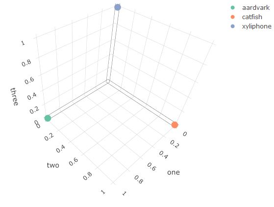
- There is one dimension for each word in the vocabulary.
- Typical vocab size = ~60k words
- All of the words are equidistant from each other.
- This is true for more dimensions.
- Similarity/relationships cannot be represented at all in this space.
We need a richer representation of these concepts to enable computers to reason about things more similarly to the way we do. One way to do this is to match each word with a distributed representation of the word. An example would be to measure our three words along a different dimension than the letters that make them up. We’ll do it with two dimensions: animalness and playability.
Representing each word on these scales produces the following:
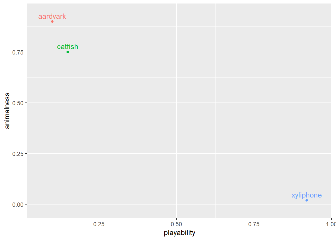
This representation has several advantages over the first:
- Dimensionality is no longer the number of words in vocab
- Words that are similar to each other in meaning are also close to each other in the distributed representation
- Aardvark and catfish both score high on the animalness dimension, so they are closer together than a xylophone.
- This nuance allows us to capture latent concepts that connect words together in the structure of the representation.
One issue is that while its easy to write code that can one hot encode any size vocabulary, it isn’t obvious how to build the representation we showed above without painstakingly thinking about every category by which we could define something. Is an Aardvark more of an animal than a goldfish? How many other ways can we slice each concept? Enter Word2Vec.
Word2Vec
The Word2Vec algorithm was developed for building vector representations of words. It operates under a simple principal: a word should be defined by it’s context. It accomplishes this by scanning over a span of words and building a model that predicts a given word from the words that surround it 3.
If you’re interested in how this algorithm works, check out this excellent blog post.
The advantages that the Word2Vec algorithm and the resulting distributed representations lends to natural language processing would also be especially valuable for our graph representation. If we want to use our graph nodes to do computation (rank paragraphs, search for things, predict things), we’ll need the numeric representation to:
- Capture the context of each node
- Entities who have similar roles in the document should have similar vector representations
- Capture relationships between nodes
- Entities which are closely associated (Putin and Russia, for example) should have similar embeddings
- Latent concepts should be captured.
As we have seen, the Word2Vec algorithm lends itself especially well to building representations that capture desirable qualities, but it depends heavily on the natural sequencing of language. One of the properties of language is that often times the relevance of words surrounding our target word diminishis with distance. For example, the words in the sentence you are reading right now are closely associated with the words in the previous sentence, but much less so as you scan further up and down the document.
We’ll need to find a way to generate sequences in the graph that have the same characteristics.
Graph Sequences: The Random Walk
A graph already has the properties we need built in. Each node has a set of connections, and as you travel further and further from the node, the relevance to the original node diminishes.
One way to travel through our graph is to traverse the graph via a random walk. The idea behind a random walk is simple:
- Start in a random node on the graph
- Pick an edge connected to that node
- Walk along it to the next node
- Repeat.
The path you walk can be thought of as a sequence of nodes, each one closely related to its immediate neighbors, and more and more loosely related as the walk progresses.
Additionally, by controlling certain parameters (walk length, weighted edges, starting points) we can intuitively capture different aspects of the graph. The code to accomplish this in python is straightforward. Starting with the graph we constructed in the previous blog post, here is the code we need to generate sequences from random walks through the graph:
nxG = fullMuellerG

startingNodes = nxG.nodes()
numWalks = 100000

walkLengths = np.random.normal(10, 3, numWalks).astype(int) # do walks of varying length

walks = []
for walkLen in walkLengths:
    start = random.choice(list(startingNodes)) # Start at a random node
    if nxG.degree(start) > 1: #Check if the starting node has neighbors
        walk = [start] #Start the walk
        for step in range(walkLen):
            paths = [n for n in nxG.neighbors(walk[-1])] #Get a list of edges to walk along
            walk.append(random.choice(paths)) #pick one and walk walk that way
        walks.append(walk)
Lets take a look at one of these walks to see what happened:
walks[3]
## ['Washington',
##  'par_689',
##  'Washington',
##  'par_213',
##  'Papadopoulos',
##  'par_25',
##  'Papadopoulos',
##  'par_194',
##  'Jeff',
##  'par_264',
##  'Laura DeMarco']
This walk started on the Washington node, visited a paragraph, came back, and wandered off towards Papadopoulos, finally landing at Laura Demarco. Visualizing this walk shows how the random walker traverses the graph:
In this case we do 100,000 random walks through the graph (roughly 20 per node) to generate sequences with average length = 10. setting this length to something smaller would allow for a more local representation, and setting it larger would allow for a more global representation.
Also note that our walks object is a list of walk sequences (also a list), which is precisely the input needed to train our Word2Vec model:
from gensim.models import Word2Vec
w2vModel = Word2Vec(walks, size=128, window=10, min_count=1, workers=16)
This represents each of the nodes in our graph with an n dimensional vector, where we have chosen n to be 128. The window size here can be used to control how ‘global’ our representation is. Increasing our window increases the size of the sequence considered to generate the context, allowing the representation to consider more distant connections in the graph.
Applications for Distributed Representations
What can we do with this representation? First, we can use it to find concepts and people that are similar to each other. To illustrate this, lets start with paragraph 459, which is excerpted below:
Throughout the day, members of the Transition Team continued to talk with foreign leaders about the resolution, with Flynn continuing to lead the outreach with the Russian government through Kislyak.1219 When Flynn again spoke with Kislyak, Kislyak informed Flynn that if the resolution came to a vote, Russia would not vote against it. 1220 The resolution later passed 14-0, with the United States
Getting the nodes that are most similar to par_459 is straightforward:
w2vModel.wv.most_similar('par_459')
## [('Michael Flynn Overview', 0.8426560759544373),
##  ('Michael Flynn', 0.6716177463531494),
##  ('Steve Bannon', 0.6249542236328125),
##  ('par_343', 0.5918193459510803),
##  ('par_474', 0.5842841267585754),
##  ('Flynn', 0.5826122760772705),
##  ('par_865', 0.5723687410354614),
##  ('par_393', 0.5675152540206909),
##  ('par_415', 0.5670546293258667),
##  ('par_890', 0.5580882430076599)]
The first items on the list are about Michael Flynn and here we recognize our first peice of magic: while paragraph 459 is certainly about Michael Flynn, it never actually says the words ‘Michael Flynn’.

The paragraph only refers to him by his last name (notice ‘Flynn’ is the 6th item down on the list). That means the word2vec algorithm has successfully generalized the concept of Michael Flynn without rigidly assigning a unique value.
Our vector representation of paragraph 459 allowed us to find latent connections between the various ways one could represent Michael Flynn, and ultimately developed a distributed representation that was closer to the more common use of Michael’s name throughout the document.
Perhaps we could use this system to discover other latent properties between individuals. For example, we could develop a system that would allow us to ask the following questions: What location is President Trump most associated with? Who is most closely tied to Moscow, TX? What places are at the center of the Clinton Email scandal?
A simple way to accomplish this is to find the nodes on the graph of a specific type which are most closely related to a given search term. In other words, to find out who is associated with Moscow we can start with the vector representation of Moscow, get similar nodes, and filter to those which are people nodes. With some manipulation of the graph structure, one way to accomplish this is with the following code: def conceptualizations(ent, target_type): mostSimilar = w2vModel.wv.most_similar(ent, topn=100)
def findRelatedConcepts(ent, target_type):
    mostSimilar = w2vModel.wv.most_similar(ent, topn=100)

    #mostSimilarParagraphs = [simTuple for simTuple in mostSimilar if simTuple[0].startswith('par')]
    similarDF = pd.DataFrame(mostSimilar, columns=['Label','similarity'])
    showDF = similarDF.merge(MuellerDF, on = 'Label')
    return showDF[showDF['D_type'] == target_type].head(5)
Running our function on Houston gives:
findRelatedConcepts('Moscow','PERSON')
## Label 	    similarity 	D_type 	Text
## Sater 	    0.516685 	PERSON 	Sater
## Felix Sater 0.484666 	PERSON 	Felix Sater
## Rhona 	    0.429744 	PERSON 	Rhona
A quick Google search of Felix Sater reveals that he was born in Moscow and that he was the lead for the Moscow Trump Tower project, purportedly boosting Trump’s Russian contacts. Another little known fact about Sater is that he helped Obama hunt down Osama bin Laden by providing bin Laden’s phone number.
A few more interesting findings:
- The person closest associated with ‘emails’ is Clinton.
- The place most associated with Donald Trump is Briarclif Manor, the location of one of his golf courses.
- The person most associated with ‘Hacking’ is Aleksei Sergeyevich Morenets, a russian hacker.
Wrapping Up
If you made it this far congratulations! I hope you had as much fun reading this as I did writing it. Vector representations are a powerful concept in deep learning and in some ways much of the progress in deep learning over the last few years owes itself to better and better representations of the data around us.
If you are interested in seeing how this technique could apply to other important documents drop a comment below.
- One hot encoding isn’t precisely the same thing as a symbolic reasoning system, but it does have some of the limitations. [return]
- You may say, hey, why can’t we just map each word to an integer? 1 = aardvark, 2 = catfish and so on? Unfortunately you have to be very careful how you encode things as numbers for a computer. Mapping to numbers tells the computer there is some relationship between the magnitude of the number and the meaning. It would attempt to reason about the problem by assuming that catfish is greater than aardvark, which doesn’t make much sense… [return]
- This method is called skip-gram. The inverse (predicting the surrounding words from the target word) is called continuous-bag-of-words, or CBOW [return]